Subsetting utilities
clisops comes with some utilities to perform common tasks that are either not implemented in xarray, or that are implemented but do not have the generality needed for climate science work. Here we show examples of the clisops.core.subset submodule.
[ ]:
import matplotlib.pyplot as plt
import xarray as xr

from clisops.core import subset

xr.set_options(display_style="html")

plt.style.use("seaborn")
plt.rcParams["figure.figsize"] = (13, 5)
%matplotlib inline
[ ]:
ds = xr.tutorial.open_dataset("air_temperature")
ds.coords
Coordinates:
  * lat      (lat) float32 75.0 72.5 70.0 67.5 65.0 ... 25.0 22.5 20.0 17.5 15.0
  * lon      (lon) float32 200.0 202.5 205.0 207.5 ... 322.5 325.0 327.5 330.0
  * time     (time) datetime64[ns] 2013-01-01 ... 2014-12-31T18:00:00
[ ]:
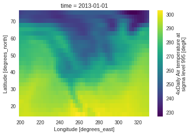
ds.air.isel(time=0).plot() # Simple index-selection with xarray
<matplotlib.collections.QuadMesh at 0x7fbce02e6760>
subset_bbox : using a latitude-longitude bounding box
In the previous example notebook, we used xarray’s .sel() to cut a lat-lon subset of our data. clisops offers the same utility, but with more generality. For example, if we mindlessly try xarray’s method on our dataset:
[ ]:
ds.sel(lat=slice(45, 50), lon=slice(-60, -55)).coords
Coordinates:
  * lat      (lat) float32
  * lon      (lon) float32
  * time     (time) datetime64[ns] 2013-01-01 ... 2014-12-31T18:00:00
As you can see, lat and lon are empty. In this dataset, the lats are defined in descending order and lons are in the range [0, 360[ instead of [-180, 180[, which is why xarray’s method did not return the expected result. clisops understands these nuances:
[ ]:
subset.subset_bbox(ds, lat_bnds=[45, 50], lon_bnds=[-60, -55]).coords
Coordinates:
  * lat      (lat) float32 50.0 47.5 45.0
  * lon      (lon) float32 300.0 302.5 305.0
  * time     (time) datetime64[ns] 2013-01-01 ... 2014-12-31T18:00:00
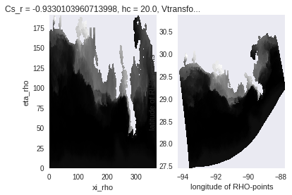
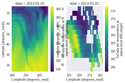
When lat and lon are 2-D
subset_bbox also manages cases where the lat-lon coordinates are not sorted 1D vectors, for example with this more complex dataset:
Most subset methods expect the input dataset / dataarray to have lat and lon as variables. It may be able to understand your data if other common names are used (like latitude, or lons), but we recommend renaming the variables before using the tool (like in this example).
[ ]:
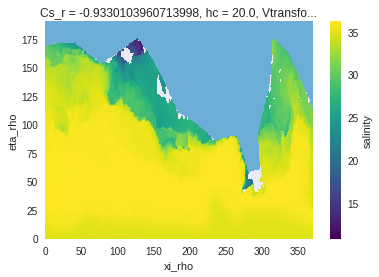
ds_roms = xr.tutorial.open_dataset("ROMS_example").rename(lon_rho="lon", lat_rho="lat")
salt = ds_roms.salt.isel(ocean_time=0, s_rho=0)

# matplotlib-based plotting
fig, (axEtaXi, axLatLon) = plt.subplots(1, 2)
salt.plot(cmap=plt.cm.gray_r, ax=axEtaXi, add_colorbar=False)
axLatLon.pcolormesh(salt.lon, salt.lat, salt)
axLatLon.set_xlabel(salt.lon.long_name)
axLatLon.set_ylabel(salt.lat.long_name)
<ipython-input-6-e7e8689dc693>:7: MatplotlibDeprecationWarning: shading='flat' when X and Y have the same dimensions as C is deprecated since 3.3.  Either specify the corners of the quadrilaterals with X and Y, or pass shading='auto', 'nearest' or 'gouraud', or set rcParams['pcolor.shading'].  This will become an error two minor releases later.
  axLatLon.pcolormesh(salt.lon, salt.lat, salt)
Text(0, 0.5, 'latitude of RHO-points')
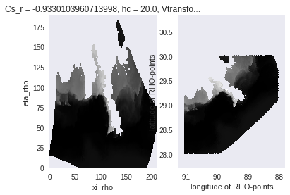
[ ]:
salt_bb = subset.subset_bbox(salt, lat_bnds=[28, 30], lon_bnds=[-91, -88])

fig, (axEtaXi, axLatLon) = plt.subplots(1, 2)
salt_bb.plot(cmap=plt.cm.gray_r, ax=axEtaXi, add_colorbar=False)
axLatLon.pcolormesh(salt_bb.lon, salt_bb.lat, salt_bb)
axLatLon.set_xlabel(salt_bb.lon.long_name)
axLatLon.set_ylabel(salt_bb.lat.long_name)
/home/phobos/Python/clisops/clisops/core/subset.py:272: UserWarning: lat and lon-like dimensions are not found among arg `<xarray.DataArray 'salt' (eta_rho: 191, xi_rho: 371)>
array([[34.953022, 34.955223, 34.957733, ..., 34.91684 , 34.913895, 34.913876],
       [34.95414 , 34.957577, 34.961086, ..., 34.916145, 34.91495 , 34.913864],
       [34.959286, 34.963936, 34.968594, ..., 34.923023, 34.92564 , 34.926853],
       ...,
       [      nan,       nan,       nan, ...,       nan,       nan,       nan],
       [      nan,       nan,       nan, ...,       nan,       nan,       nan],
       [      nan,       nan,       nan, ...,       nan,       nan,       nan]],
      dtype=float32)
Coordinates:
    Cs_r        float64 ...
    lon         (eta_rho, xi_rho) float64 -93.6 -93.58 -93.57 ... -88.88 -88.87
    hc          float64 ...
    h           (eta_rho, xi_rho) float64 ...
    lat         (eta_rho, xi_rho) float64 27.45 27.45 27.45 ... 30.85 30.86
    Vtransform  int32 ...
    ocean_time  datetime64[ns] 2001-08-01
    s_rho       float64 -0.9833
Dimensions without coordinates: eta_rho, xi_rho
Attributes:
    long_name:  salinity
    time:       ocean_time
    field:      salinity, scalar, series` dimensions: ['eta_rho', 'xi_rho'].
  warnings.warn(
<ipython-input-7-67bc17b9a9a6>:5: MatplotlibDeprecationWarning: shading='flat' when X and Y have the same dimensions as C is deprecated since 3.3.  Either specify the corners of the quadrilaterals with X and Y, or pass shading='auto', 'nearest' or 'gouraud', or set rcParams['pcolor.shading'].  This will become an error two minor releases later.
  axLatLon.pcolormesh(salt_bb.lon, salt_bb.lat, salt_bb)
Text(0, 0.5, 'latitude of RHO-points')
Add time subsetting
subset_bbox and other methods of the submodule give options to also give time bounds. These options are mostly for convenience as only some basics sanity checks are performed.
[ ]:
subset.subset_bbox(ds, lat_bnds=[45, 50], lon_bnds=[-60, -55], start_date="2013-02", end_date="2013-08").coords
Coordinates:
  * lat      (lat) float32 50.0 47.5 45.0
  * lon      (lon) float32 300.0 302.5 305.0
  * time     (time) datetime64[ns] 2013-02-01 ... 2013-08-31T18:00:00
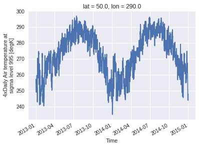
subset_gridpoint : Selecting grid points
subset_gridpoint can be used for selecting single locations. Compared to .sel(), this method adds a tolerance parameter in meters so that it finds the nearest point from the given coordinate within this distance, or else it returns NaN.
[ ]:
lon_pt = -70.2
lat_pt = 50.1

# Get timeseries for point within 100 km of (-70.2, 50.1)
ds3 = subset.subset_gridpoint(ds, lon=lon_pt, lat=lat_pt, tolerance=100 * 1000)
ds3.coords
Coordinates:
    lat      float32 50.0
    lon      float32 290.0
  * time     (time) datetime64[ns] 2013-01-01 ... 2014-12-31T18:00:00
[ ]:
ds3.air.plot()
[<matplotlib.lines.Line2D at 0x7fbcdfc62b20>]
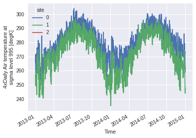
This also works with a list of coordinates. In that case, a new dimension site concatenates the selected gridpoints. Moreover, passing add_distance = True allows us to inspect how close the selected gridpoints were from the requested coordinates. In this example, the third point (-90, 54.1) is a little bit further than 100 km from the nearest gridpoint, so the coordinate of this gridpoint and the distance are returned, but the values are masked with NaN (and thus they do not appear on
the graph).
[ ]:
lon_pt = [-65, -70.2, -90]
lat_pt = [45, 50.1, 54.1]

# Get timeseries for point within 100 km of each points
ds3 = subset.subset_gridpoint(ds, lon=lon_pt, lat=lat_pt, tolerance=100 * 1000, add_distance=True)
print(ds3.coords)
ds3.air.plot(hue="site")
Coordinates:
    lat       (site) float32 45.0 50.0 55.0
    lon       (site) float32 295.0 290.0 270.0
  * time      (time) datetime64[ns] 2013-01-01 ... 2014-12-31T18:00:00
    distance  (site) float64 0.0 1.814e+04 1.002e+05
[<matplotlib.lines.Line2D at 0x7fbcdfb2fa60>,
 <matplotlib.lines.Line2D at 0x7fbcdfb66490>,
 <matplotlib.lines.Line2D at 0x7fbcdfb66310>]
subset_shape : Selecting a region from a polygon
If the region we want to keep in our dataset is complex, we can use subset_shape and pass a polygon. The input shape can be any georeferenced data file understood by geopandas and fiona that run under the hood. For example here with a geojson file of Canada available online:
[ ]:
ds_can = subset.subset_shape(ds, "https://raw.githubusercontent.com/johan/world.geo.json/master/countries/CAN.geo.json")

fig, (axall, axcan) = plt.subplots(1, 2)
ds.air.isel(time=0).plot(ax=axall)
ds_can.air.isel(time=0).plot(ax=axcan)
2021-01-26 14:44:38,120 - root - INFO - No file or no dimensions found in arg `https://raw.githubusercontent.com/johan/world.geo.json/master/countries/CAN.geo.json`.
/home/phobos/Python/clisops/clisops/core/subset.py:279: UserWarning: CRS definitions are similar but raster lon values must be wrapped.
  final = func(*formatted_args, **kwargs)
/home/phobos/Python/clisops/clisops/core/subset.py:463: UserWarning: Wrapping longitudes at 180 degrees.
  warnings.warn("Wrapping longitudes at 180 degrees.")
<matplotlib.collections.QuadMesh at 0x7fbcdf949310>
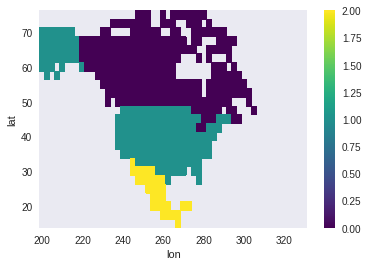
create_mask : Creating a mask from polygons
We can also create a mask to divide the data in regions. In the example, we load the shapes for Canada, Mexico and the US, merge them with pandas and then create the mask. create_mask is a bit more restrictive than the other methods showed here and specifically asks for the x and y dims. Also, we need to pass wrap_lons=True since our longitudes go from 0 to 360 instead of -180 to 180.
[ ]:
import geopandas as gpd
import pandas as pd

can = gpd.read_file("https://raw.githubusercontent.com/johan/world.geo.json/master/countries/CAN.geo.json")
usa = gpd.read_file("https://raw.githubusercontent.com/johan/world.geo.json/master/countries/USA.geo.json")
mex = gpd.read_file("https://raw.githubusercontent.com/johan/world.geo.json/master/countries/MEX.geo.json")
northam = pd.concat([can, usa, mex]).set_index("id")
northam
| name | geometry | |
|---|---|---|
| id | ||
| CAN | Canada | MULTIPOLYGON (((-63.66450 46.55001, -62.93930 ... |
| USA | United States of America | MULTIPOLYGON (((-155.54211 19.08348, -155.6881... |
| MEX | Mexico | POLYGON ((-97.14001 25.87000, -97.52807 24.992... |
[ ]:
mask = subset.create_mask(x_dim=ds.lon, y_dim=ds.lat, poly=northam, wrap_lons=True)
/home/phobos/Python/clisops/clisops/core/subset.py:463: UserWarning: Wrapping longitudes at 180 degrees.
  warnings.warn("Wrapping longitudes at 180 degrees.")
[ ]:
mask.T.plot() # The transpose is needed because create_mask returns lon, lat instead the input lat, lon.
<matplotlib.collections.QuadMesh at 0x7fbcdf82ad00>
The same can be done with 2D lat/lon coordinates. Here get the regions of salt that are within the boundaries of the US as defined in our geojson data. As our data comes from a small region in the Gulf of Mexico and our USA mask is quite coarse, the following isn’t really helpful. In any case, it illustrates what can be done with clisops.
[ ]:
usa_mask = subset.create_mask(x_dim=salt.lon, y_dim=salt.lat, poly=usa)
[ ]:
salt.plot()
usa_mask.plot(cmap=plt.cm.Blues_r, add_colorbar=False)
<matplotlib.collections.QuadMesh at 0x7fbcdf778df0>
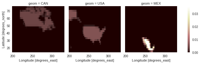
create_weight_masks : Creating exact weights masks from polygons
While create_mask (and subset_shape) only check if the center of a grid cell lies inside of a polygon or not, create_weight_masks (and average_shape, see the Average utilities notebook) consider the partial overlap of grid cells and polygons. Thus, instead of creating an integer mask for the data, this method creates one mask for each polygon. The weights are the fraction of the grid cells-polygon overlap over the whole polygon. As such, the sum along spatial dimensions gives 1
for each geometry.
However, this feature of clisops requires the optional xESMF dependency (version 0.6.2 or later), which is not currently available of pypi (pip) and must be installed either through conda or from the source.
The call signature is different: a dataset or dataarray containing the grid information is passed directly. The same restrictions as for xESMF apply.
[ ]:
weights = subset.create_weight_masks(ds, northam)
weights
<xarray.DataArray (geom: 3, lat: 25, lon: 53)>
array([[[0.00000000e+00, 0.00000000e+00, 0.00000000e+00, ...,
         0.00000000e+00, 0.00000000e+00, 0.00000000e+00],
        [0.00000000e+00, 0.00000000e+00, 0.00000000e+00, ...,
         0.00000000e+00, 0.00000000e+00, 0.00000000e+00],
        [0.00000000e+00, 0.00000000e+00, 0.00000000e+00, ...,
         0.00000000e+00, 0.00000000e+00, 0.00000000e+00],
        ...,
        [0.00000000e+00, 0.00000000e+00, 0.00000000e+00, ...,
         0.00000000e+00, 0.00000000e+00, 0.00000000e+00],
        [0.00000000e+00, 0.00000000e+00, 0.00000000e+00, ...,
         0.00000000e+00, 0.00000000e+00, 0.00000000e+00],
        [0.00000000e+00, 0.00000000e+00, 0.00000000e+00, ...,
         0.00000000e+00, 0.00000000e+00, 0.00000000e+00]],

       [[0.00000000e+00, 0.00000000e+00, 0.00000000e+00, ...,
         0.00000000e+00, 0.00000000e+00, 0.00000000e+00],
        [0.00000000e+00, 4.38326936e-05, 1.38383820e-05, ...,
         0.00000000e+00, 0.00000000e+00, 0.00000000e+00],
        [4.47662669e-03, 5.31807679e-03, 5.29956131e-03, ...,
         0.00000000e+00, 0.00000000e+00, 0.00000000e+00],
...
        [0.00000000e+00, 1.73510030e-04, 9.35640399e-04, ...,
         0.00000000e+00, 0.00000000e+00, 0.00000000e+00],
        [0.00000000e+00, 0.00000000e+00, 0.00000000e+00, ...,
         0.00000000e+00, 0.00000000e+00, 0.00000000e+00],
        [0.00000000e+00, 0.00000000e+00, 0.00000000e+00, ...,
         0.00000000e+00, 0.00000000e+00, 0.00000000e+00]],

       [[0.00000000e+00, 0.00000000e+00, 0.00000000e+00, ...,
         0.00000000e+00, 0.00000000e+00, 0.00000000e+00],
        [0.00000000e+00, 0.00000000e+00, 0.00000000e+00, ...,
         0.00000000e+00, 0.00000000e+00, 0.00000000e+00],
        [0.00000000e+00, 0.00000000e+00, 0.00000000e+00, ...,
         0.00000000e+00, 0.00000000e+00, 0.00000000e+00],
        ...,
        [0.00000000e+00, 0.00000000e+00, 0.00000000e+00, ...,
         0.00000000e+00, 0.00000000e+00, 0.00000000e+00],
        [0.00000000e+00, 0.00000000e+00, 0.00000000e+00, ...,
         0.00000000e+00, 0.00000000e+00, 0.00000000e+00],
        [0.00000000e+00, 0.00000000e+00, 0.00000000e+00, ...,
         0.00000000e+00, 0.00000000e+00, 0.00000000e+00]]])
Coordinates:
    name     (geom) object 'Canada' 'United States of America' 'Mexico'
  * geom     (geom) object 'CAN' 'USA' 'MEX'
  * lat      (lat) float32 75.0 72.5 70.0 67.5 65.0 ... 25.0 22.5 20.0 17.5 15.0
* lon (lon) float32 200.0 202.5 205.0 207.5 ... 322.5 325.0 327.5 330.0- geom: 3
- lat: 25
- lon: 53
- 0.0 0.0 0.0 0.0 0.0 0.0 0.0 0.0 ... 0.0 0.0 0.0 0.0 0.0 0.0 0.0 0.0
array([[[0.00000000e+00, 0.00000000e+00, 0.00000000e+00, ..., 0.00000000e+00, 0.00000000e+00, 0.00000000e+00], [0.00000000e+00, 0.00000000e+00, 0.00000000e+00, ..., 0.00000000e+00, 0.00000000e+00, 0.00000000e+00], [0.00000000e+00, 0.00000000e+00, 0.00000000e+00, ..., 0.00000000e+00, 0.00000000e+00, 0.00000000e+00], ..., [0.00000000e+00, 0.00000000e+00, 0.00000000e+00, ..., 0.00000000e+00, 0.00000000e+00, 0.00000000e+00], [0.00000000e+00, 0.00000000e+00, 0.00000000e+00, ..., 0.00000000e+00, 0.00000000e+00, 0.00000000e+00], [0.00000000e+00, 0.00000000e+00, 0.00000000e+00, ..., 0.00000000e+00, 0.00000000e+00, 0.00000000e+00]], [[0.00000000e+00, 0.00000000e+00, 0.00000000e+00, ..., 0.00000000e+00, 0.00000000e+00, 0.00000000e+00], [0.00000000e+00, 4.38326936e-05, 1.38383820e-05, ..., 0.00000000e+00, 0.00000000e+00, 0.00000000e+00], [4.47662669e-03, 5.31807679e-03, 5.29956131e-03, ..., 0.00000000e+00, 0.00000000e+00, 0.00000000e+00], ... [0.00000000e+00, 1.73510030e-04, 9.35640399e-04, ..., 0.00000000e+00, 0.00000000e+00, 0.00000000e+00], [0.00000000e+00, 0.00000000e+00, 0.00000000e+00, ..., 0.00000000e+00, 0.00000000e+00, 0.00000000e+00], [0.00000000e+00, 0.00000000e+00, 0.00000000e+00, ..., 0.00000000e+00, 0.00000000e+00, 0.00000000e+00]], [[0.00000000e+00, 0.00000000e+00, 0.00000000e+00, ..., 0.00000000e+00, 0.00000000e+00, 0.00000000e+00], [0.00000000e+00, 0.00000000e+00, 0.00000000e+00, ..., 0.00000000e+00, 0.00000000e+00, 0.00000000e+00], [0.00000000e+00, 0.00000000e+00, 0.00000000e+00, ..., 0.00000000e+00, 0.00000000e+00, 0.00000000e+00], ..., [0.00000000e+00, 0.00000000e+00, 0.00000000e+00, ..., 0.00000000e+00, 0.00000000e+00, 0.00000000e+00], [0.00000000e+00, 0.00000000e+00, 0.00000000e+00, ..., 0.00000000e+00, 0.00000000e+00, 0.00000000e+00], [0.00000000e+00, 0.00000000e+00, 0.00000000e+00, ..., 0.00000000e+00, 0.00000000e+00, 0.00000000e+00]]]) - name(geom)object'Canada' ... 'Mexico'
array(['Canada', 'United States of America', 'Mexico'], dtype=object)
- geom(geom)object'CAN' 'USA' 'MEX'
array(['CAN', 'USA', 'MEX'], dtype=object)
- lat(lat)float3275.0 72.5 70.0 ... 20.0 17.5 15.0
- standard_name :
- latitude
- long_name :
- Latitude
- units :
- degrees_north
- axis :
- Y
array([75. , 72.5, 70. , 67.5, 65. , 62.5, 60. , 57.5, 55. , 52.5, 50. , 47.5, 45. , 42.5, 40. , 37.5, 35. , 32.5, 30. , 27.5, 25. , 22.5, 20. , 17.5, 15. ], dtype=float32) - lon(lon)float32200.0 202.5 205.0 ... 327.5 330.0
- standard_name :
- longitude
- long_name :
- Longitude
- units :
- degrees_east
- axis :
- X
array([200. , 202.5, 205. , 207.5, 210. , 212.5, 215. , 217.5, 220. , 222.5,
       225. , 227.5, 230. , 232.5, 235. , 237.5, 240. , 242.5, 245. , 247.5,
       250. , 252.5, 255. , 257.5, 260. , 262.5, 265. , 267.5, 270. , 272.5,
       275. , 277.5, 280. , 282.5, 285. , 287.5, 290. , 292.5, 295. , 297.5,
       300. , 302.5, 305. , 307.5, 310. , 312.5, 315. , 317.5, 320. , 322.5,
       325. , 327.5, 330. ], dtype=float32)
[ ]:
weights.plot(col="geom", cmap="pink")
<xarray.plot.facetgrid.FacetGrid at 0x7fbcddd3f640>
[ ]:
weights.sum(["lon", "lat"])
<xarray.DataArray (geom: 3)>
array([1., 1., 1.])
Coordinates:
    name     (geom) object 'Canada' 'United States of America' 'Mexico'
* geom (geom) object 'CAN' 'USA' 'MEX'- geom: 3
- 1.0 1.0 1.0
array([1., 1., 1.])
- name(geom)object'Canada' ... 'Mexico'
array(['Canada', 'United States of America', 'Mexico'], dtype=object)
- geom(geom)object'CAN' 'USA' 'MEX'
array(['CAN', 'USA', 'MEX'], dtype=object)